Methodology
Methodology
Here are the steps taken for our project.
Data Collection
For the purpose of this project, we retrieved data from the following sources:
- The co-ordinates of the TEL Stage 4 train stations via GeoHack. These co-ordinates consist of the latitude and longitude of each train station which is needed to plot the points in QGIS for analysis.
- OSM (Geofabrik). We needed to extract walkway and building features for our analysis.
- Population data from SingStat. This is needed to derive the population density as part of our analysis.
- Bus Stop co-ordinates from LTA DataMall.
Data Plotting
Based on the train station co-ordinates retrieved from GeoHack, we saved it in a CSV file with the following column name:
station_code
station_name
latitude
longitude
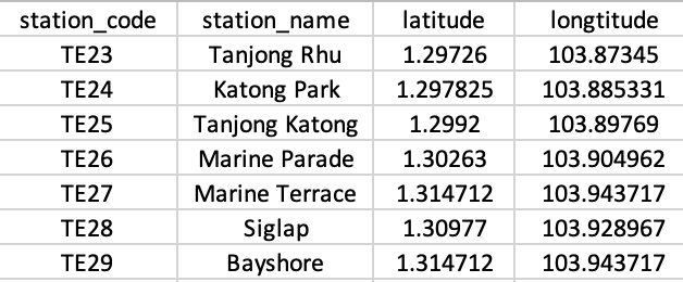
Subsequently, we imported this CSV file into QGIS by adding it as a new delimited text layer.
After these features have been plotted and is shown correctly on the map, we saved them into the LandUse GeoPackage.
Data Extraction
Walkway Features
The OSM Road layer contains several types of roads that are not relevant to our analysis, which explains the need to extract only the required road types in QGIS.
Based on our research on the types of roads that residents are most likely to walk on, here is the list of road types that are of interest to us:
Cycleway.
Footway.
Living Street.
Path.
Pedestrian.
Steps.
Thereafter, we created the expression used to extract these features from the OSM layer:
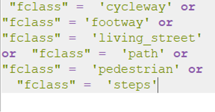
After these features have been selected, we saved them into the LandUse GeoPackage.
Residential Building Features
The OSM Building layer contains several types of buildings that are not relevant to our analysis, which explains the need to extract only the required building types in QGIS.
Based on our research on the types of buildings that residents are most likely to stay in, here is the list of building types that are of interest to us:
Apartments.
Bungalow.
Condominium.
Detached.
Dormitory.
House.
Residential.
Semidetached House.
Terrace.
Thereafter, we created the expression used to extract these features from the OSM layer:
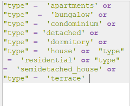
After these features have been selected, we saved them into the LandUse GeoPackage. One assumption we had to make was finding the population of residences without having an actual population data of residences living within the catchment area. Hence we created another new field called BuildingType which we further classified our residential building data into 3 different building types:
Terrace
Condo
HDB
This enabled us to label the population of an average household living in each building type based on the availability of information regarding people living in condos, HDBs and terrace houses in Singapore when we are estimating the residential population.
Bus Stops
As we wanted to analyse public transport accessibility, we took into account the number of bus stops that fall within the catchment area of each TEL train station. In order to so, we downloaded the bus stop location shape file from LTA Data Mall.
Subsequently, we imported the bus stop shape file into our project and used the Clip function to delineate the bus stops that fall within the catchment areas of each TEL train stations.
Creating the Catchment
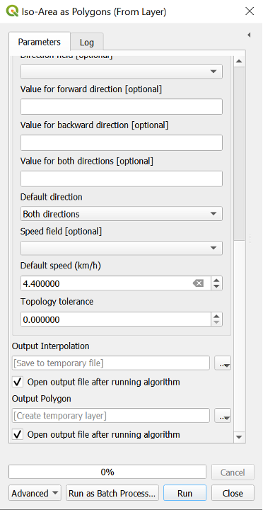
We delineated the catchment area for each TEL train station using the QNEAT3 plugin.
The distance was set to 500m, while the walking speed was set at 4.4 km/h.
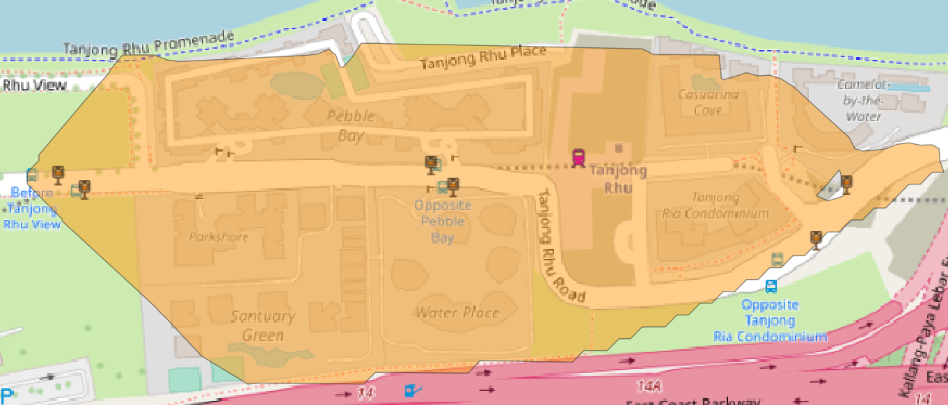
This process was done individually for each train station, starting with the first train station TE23 Tanjong Rhu Station.
It is important that this catchment is created per train station by ensuring that only one train station is selected in QGIS before creating the catchment.
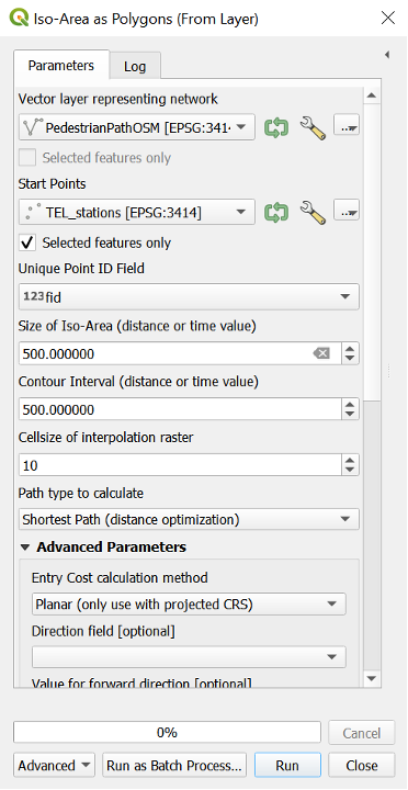
An example of a catchment area created in orange (TE23 Tanjong Rhu Station):
Estimating the Residential Population
The total residential population in the catchment area was derived by summing up all the residential population in the respective catchment areas.
Based on the data gathered from SingStat, we estimated the number of people living in each residential type:
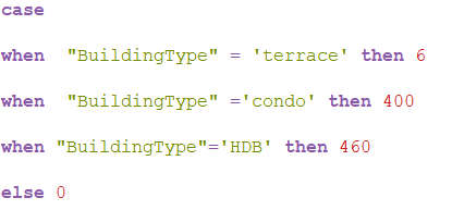
HDB: 640 people per block.
Condominiums: 400 people per block.
Terrace: 6 people per landed unit.
For example, based on our research, there are currently 38 blocks of condo in the vicinity of TE23 Tanjong Rhu Station which houses about 400 residents per block. Hence, the total estimated population is about 15,200 residents living in the catchment area of TE23. We then went on to populate the residential building types based on our estimation using the following expression:
This process was done for all the TEL train stations.
Population Density Formula
The formula that we used to derive the population density is as follow:
\[ \frac{Total \; Residential \; Population \; in \; Catchment \; Area } {Total \;Catchment \; Area} \]
Calculating the Geographical Area
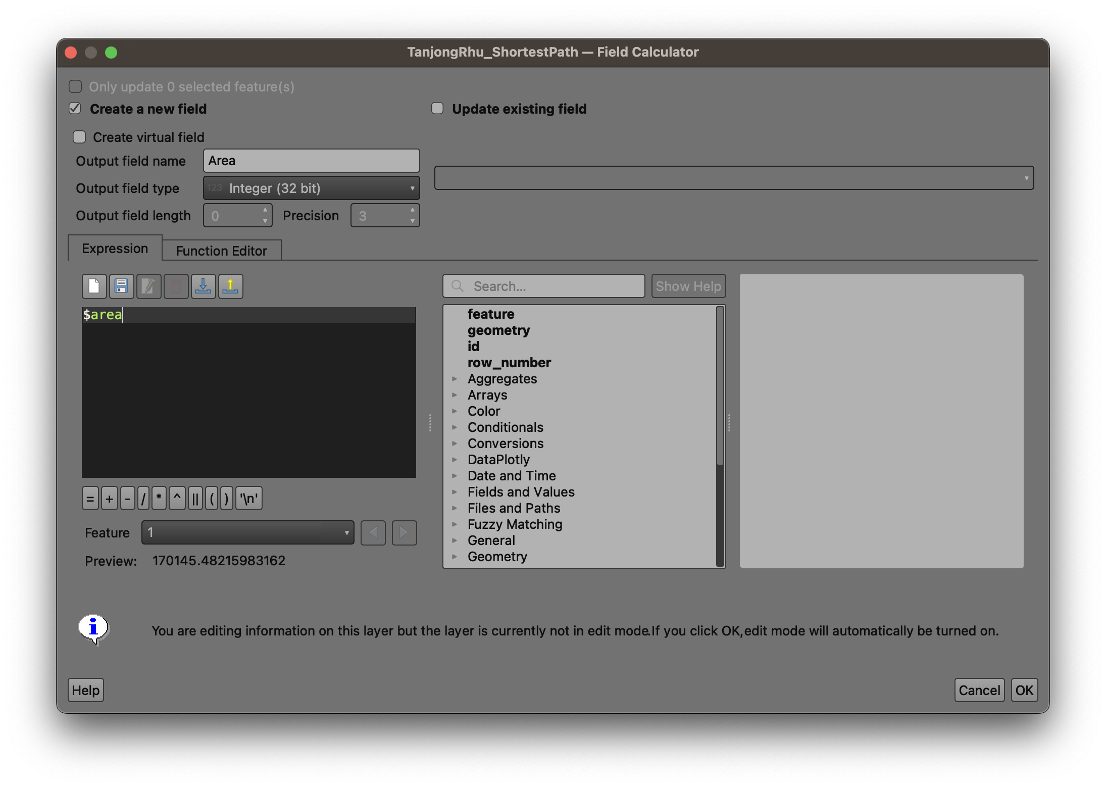
The total catchment area was calculated via QGIS’s in-built field calculator using the expression $area.
For example, for TE23 Tanjong Rhu Station, we opened the Attribute Table and created a new column called ‘Area’ using the aforementioned expression. This would generate the size of the catchment area in square meters. In this example, the area of TE23 is 170,145 square meters.
Calculating the Population Density
After we have derived the residential number and the size of the catchment area, we are able to derive the population density of the catchment area using the formula listed in the earlier section.
A new column called PopDensity was created for each TEL catchment area.

In the case of TE23 Tanjong Rhu Station which has a residential population of 15,200 and a catchment area size of 170,145, the calculation would be:
\[ \frac{15,200} {170,145} = 0.089333 \]
Similarly, this process and calcuation was done for the remaining TEL Stage 4 train stations. The full list of population density for each train station can be found here in our analysis.